NFL Predictions
Amazon product co-purchasing network
Data
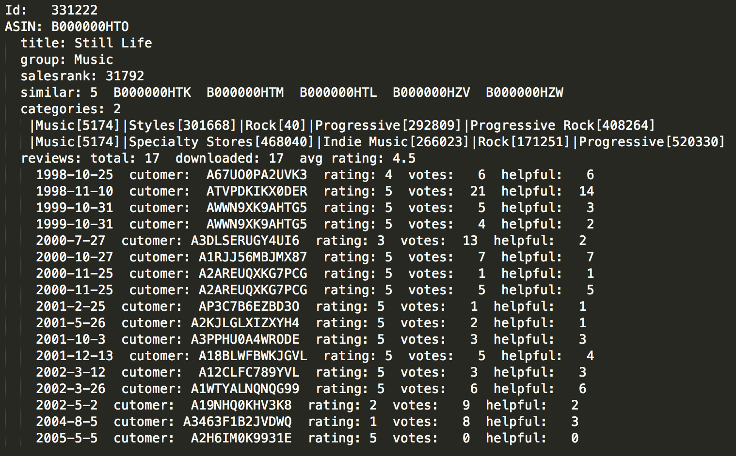
The data selected for this analysis has information about products sold in Amazon during the summer of 2006. It has four types of products: books, DVDs, CDs and Videos. For each product the data provides title, sales rank, list of similar products, category and product review including individual ratings from users. This link would allow to create the user to product network. For the users we have the rating the user gave to a given product and if the rating was of help to other users. In total there are 548,552 nodes and 1,788,725 edges in the data. The most direct edge provided by the data is the field similar. However this field is limited to 5 products.
Data preprocessing
The data structure is unstructured and since it is likely to be used many times for sampling, a master file with a more accessible format was created. The attributes in the master file are the following: ASIN (Amazon’s product id), title, product type (book, DVDs, etc), number of co-purchased products, ASIN of co-purchased products, average rating, users id and user’s rating. Having this master allow me to use it for additional experiments where I am implementing Hadoop to perform queries to build additional samples.
To handle and process the data more efficiently the master file was divided into 6 chunks with 100k products in each file. The data was filtered only by degree so I may be able to find communities of users that buy books, music or videos. My hope would be to have many users that have rated multiple products so that I may have a more connected local networks. I would expect to have two types of relevant nodes. One of them would have high degree and another high betweenness (to identify communities). The edges are set by the products that are being purchased together. The edges weights could be the rating provided by the user to each product.
Sampling & Filtering
The number of nodes and edges is so vast that it is necessary to filter the data. With the data structured in a more accessible the next step is to reduce the dimension of the data. The initial approach was to create random samples using all types of products. Many samples were created trying to see consistency in the results and if it was possible to detect communities of users that have tendencies to get books, or CDS or any other product in the network. However the network space is large and the random approach yield bad results. To solve this issue another approach was implemented, Snowball sampling. This approach may return bias networks since the sample is created by selecting a node and capture its connections until the size of the network is has a right size for analysis. Is easy to implement and in cases like these where time is a constraint is a good approach.
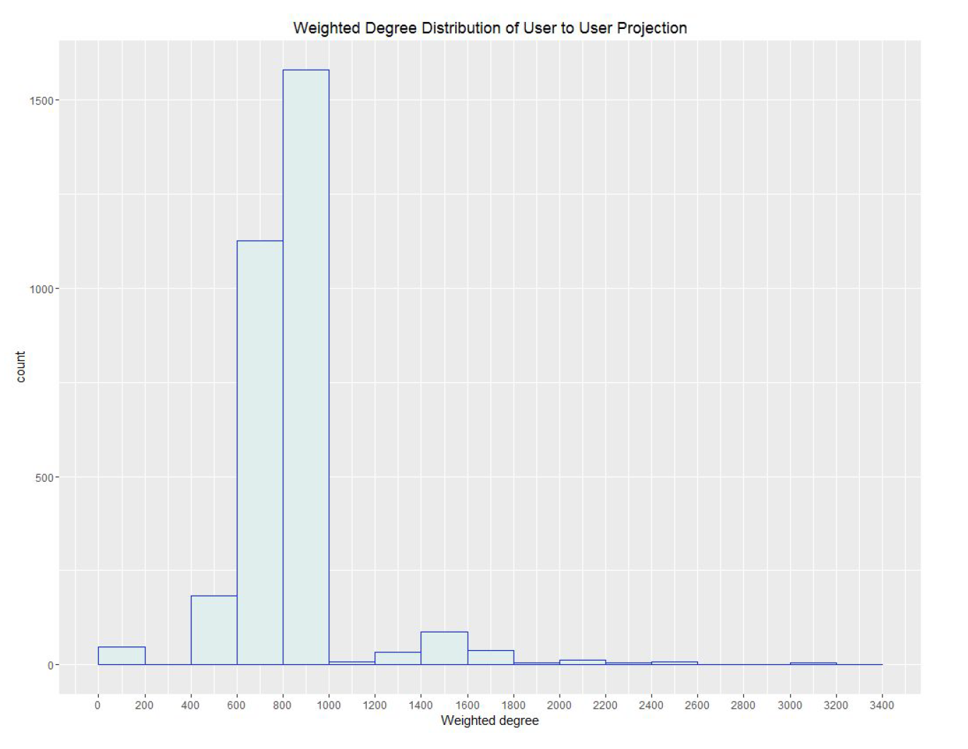
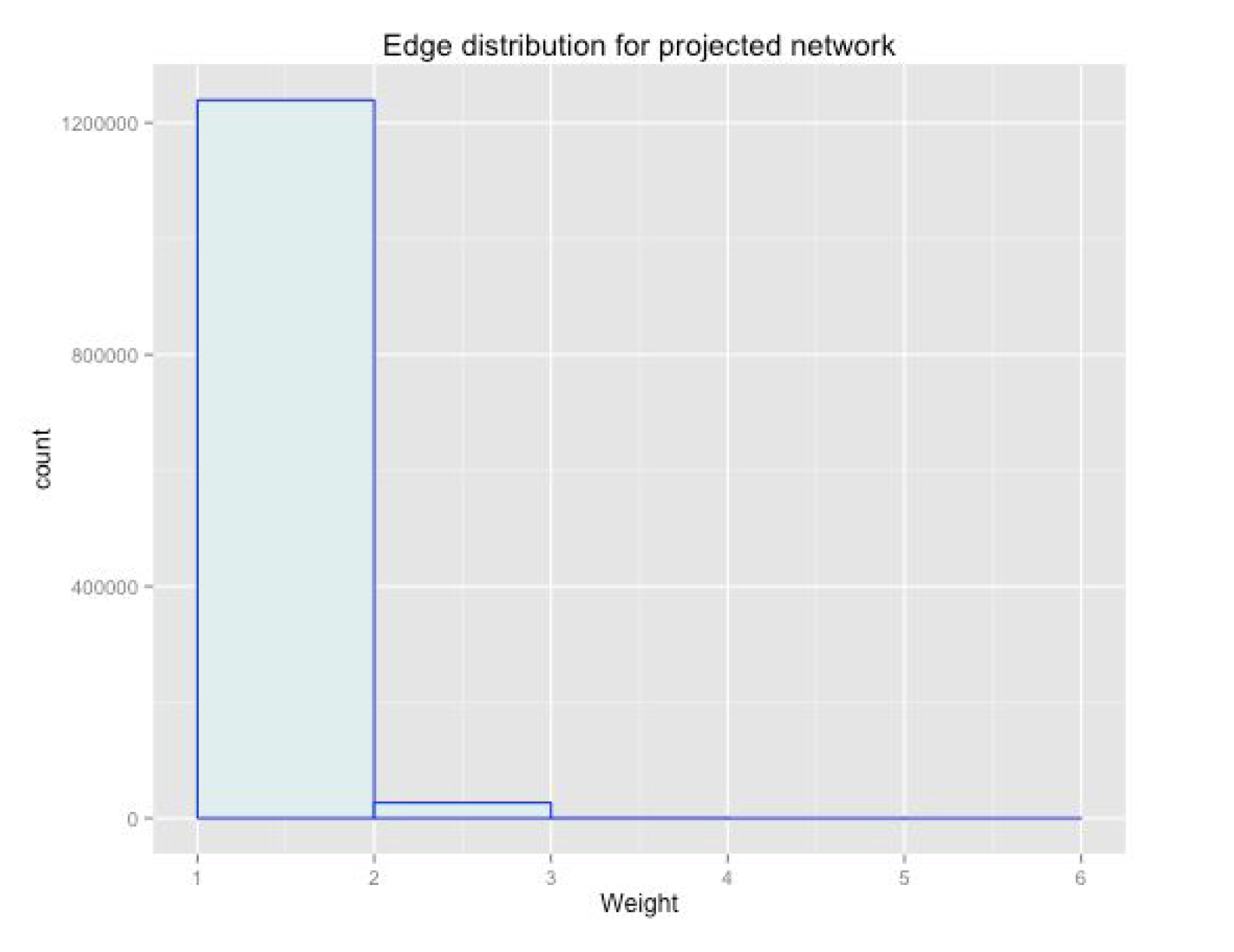
The initial node for the sample created is the book “Max Notes – To Kill a Mockingbird (MAXnotes)”. The reason to select this book is because is related to the popular novel from Harper Lee, and it has 1,410 ratings. Since the edges of the bipartite network are created using the field similar items of the products having a lar number of users is helpful have more probabilities of having a more dense user to user projection. The sample was grow until it reach 8 products. All of them turn out to be books. The number of ratings capture by this sample is 5,329 from 3,139 different users. The projection of user to user produces a total of 1,266,475 edges. The weighted degree distribution shown in appendix A3, show a dense network with a large right tail. In addition the weighted edge distribution of the resulting network, shown in appendix A4, show a power law distribution. Denoting some highly connected users .
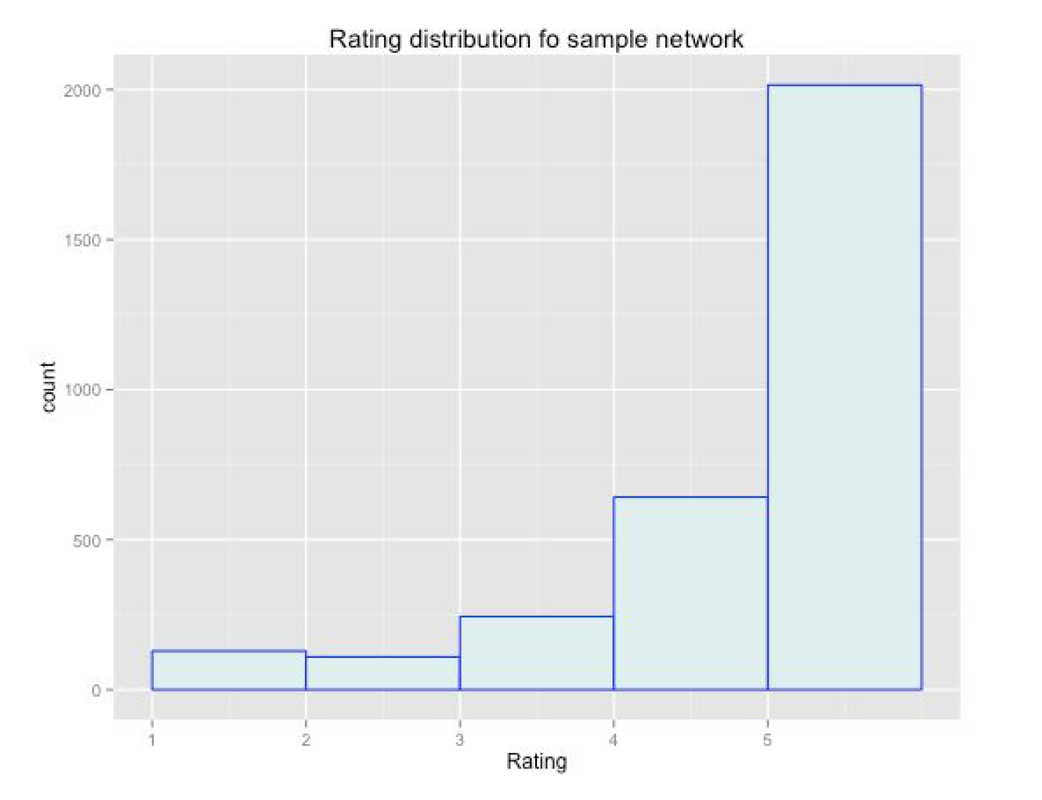
In order to get a sample that is possible to analyse more closely filtering is applied. The first step was to delete edges that had weight lower than 3, keeping weight up to 6. This filter produce singletons that can be removed by updating degree and deleting those equal to zero. The final number of nodes is 53 with 405 edges. One final distribution shown in appendix A5 is the rating provided by the users. This distribution has a long left tail, more frequently users in the network gave really high ratings
Analysis
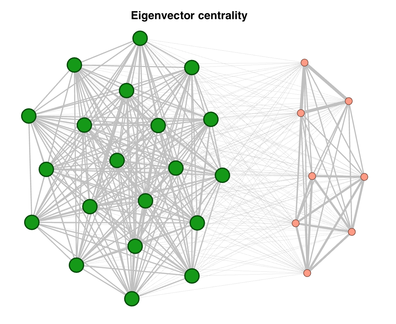
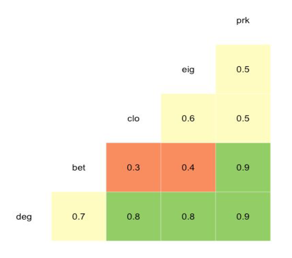
We need to identify what an important node is. Using centrality measures it’s possible to identify different relations among the vertices. Allowing to get an idea of what may be defined as a relevant node. From the centrality measures the data indicates that the projection of the user to user network has a high correlation between degree and closeness. That means that a highly connected user has short paths to the network, already expected. The eigenvector centrality talks about how neighbors are positions that are likely to have high degree neighbors. That implies high degree correlation, and the sample capture by snowball is highly concentrated among users with high degree. Betweenness is not highly correlated to any of the other measures as expected by the sampling approach. But that also means that there must be some users that have bought products in a wide range of categories that allow to build networks that otherwise may not exist.
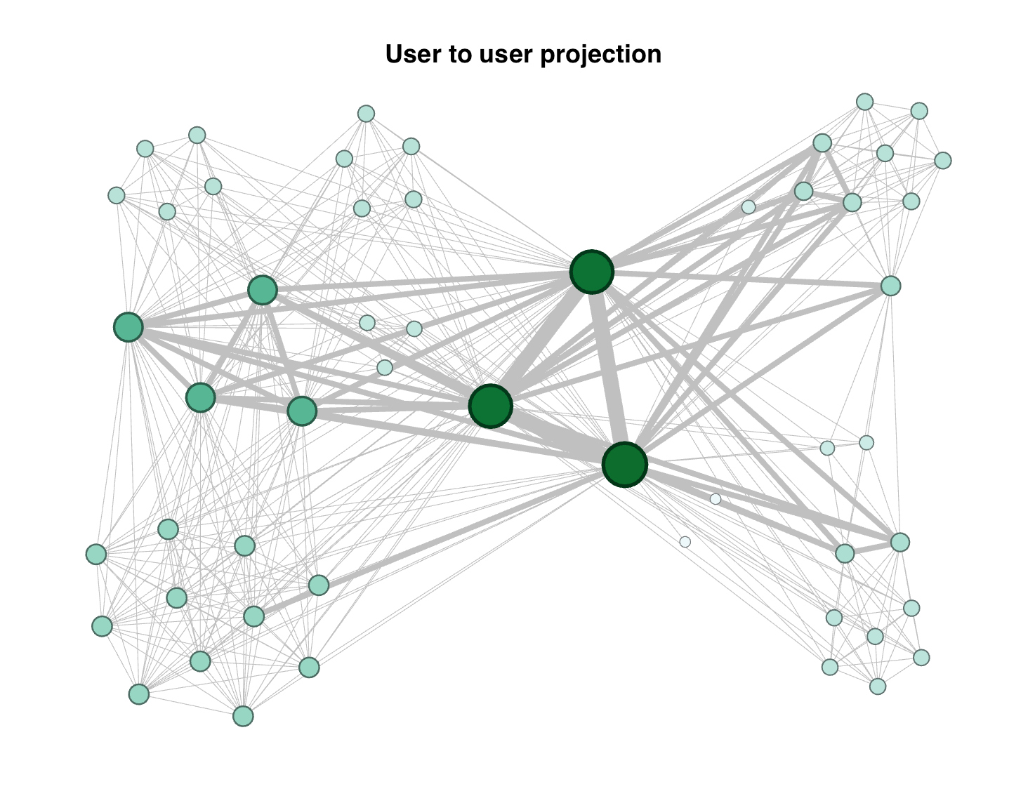
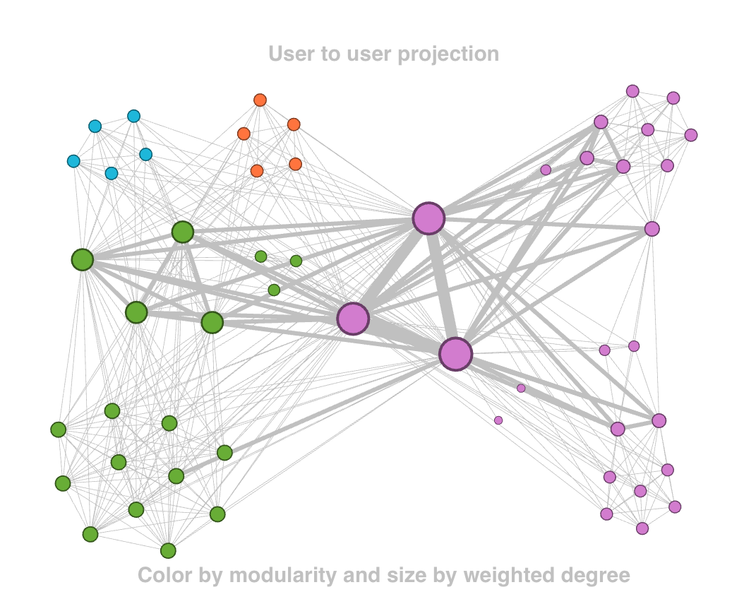
Looking at the first visualization of the user to user projection we see what was expected from the previous analysis. The network is concentrated among highly connected users. The node sizes are set to the weighted degree and color is set to betweenness. The network shows in dark green user that hold the network connected. We may also see 7 clusters around these users. Even when the clusters are dense the edges that the three main users hold are far more as observed in the distribution. We may think that this three users are wider readers. While the clusters prefer to read same type of readings. A larger size of the graph at appendix A5. There is another group of four users, located at the center-left of the image, that have high betweenness with the clusters above and below them. That tells us about another type of readers that have also different interest.
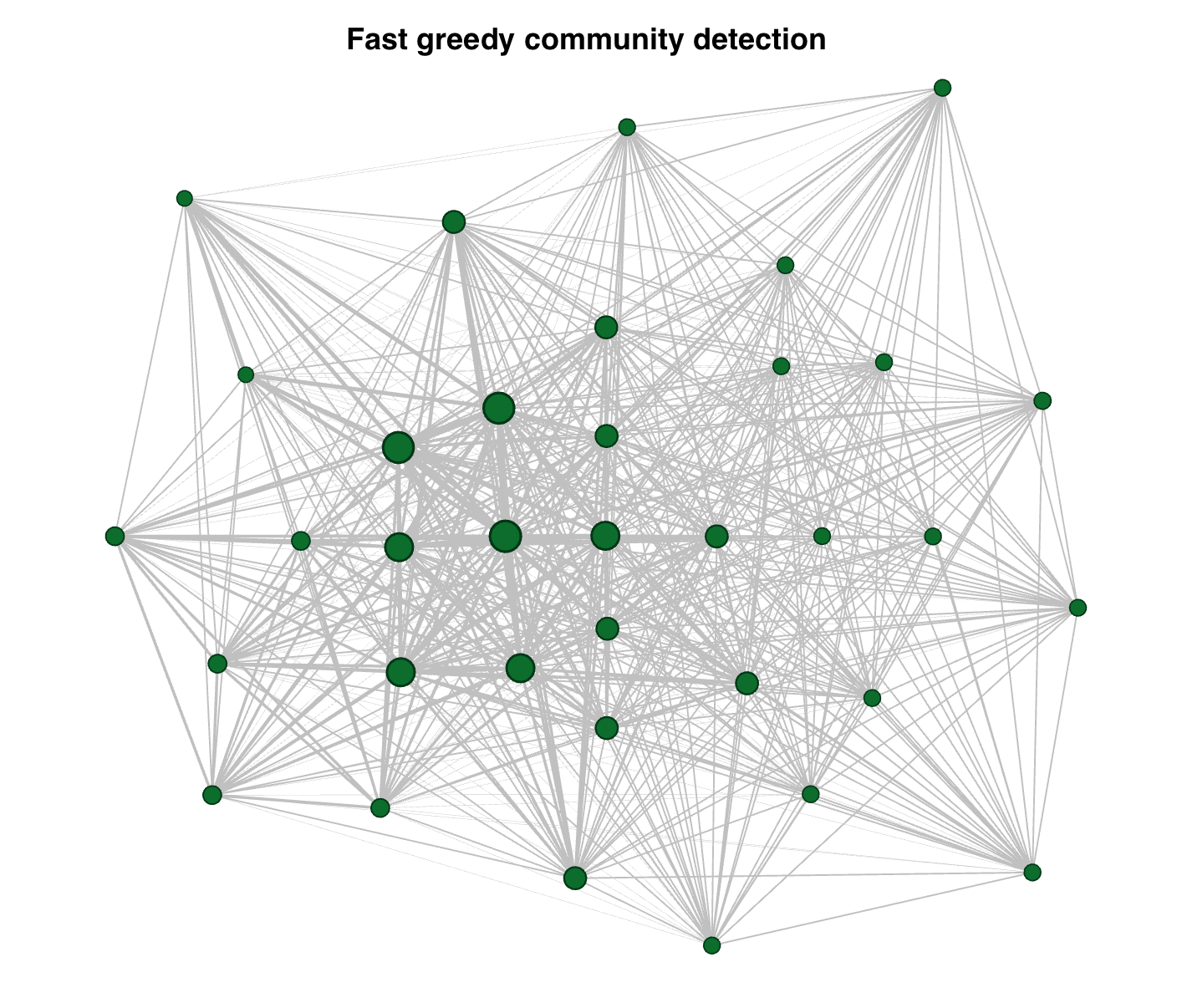
Running community detection yields what we see in filtered projected network. Using the original user to user projection community detection was performed using fast greedy, ten steps walktrap and eigenvector. Modularity values for all three are very similar. With 0.6 the lowest value is obtained with walktrap, followed by fastgreedy with 0.61 and eigenvector with the highest value of 0.62. The number of communities for the first two are 7. The same number identified in the user to user graph in the previous page. A visualization of the largest cluster is shown in appendix A6. This community as expected has high degree across the users in the cluster. Unlike the other two measure, eigenvector identifies 6 groups. However one of them could be further split. Shown in appendix A7 we see that the largest cluster identified by eigenvector may be divided into to local networks. Running modularity in gephi over this community is possible to recreate the image shown.
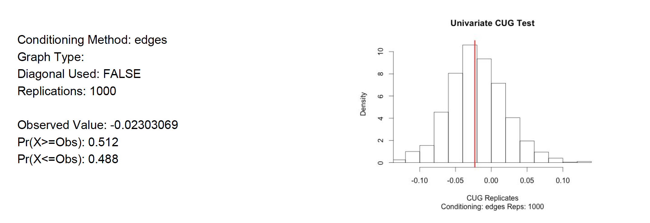
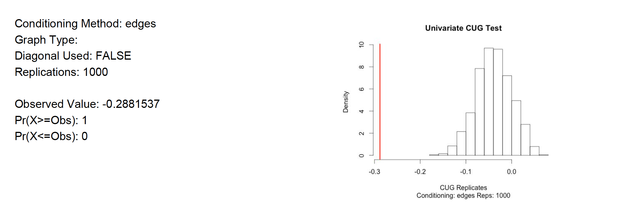
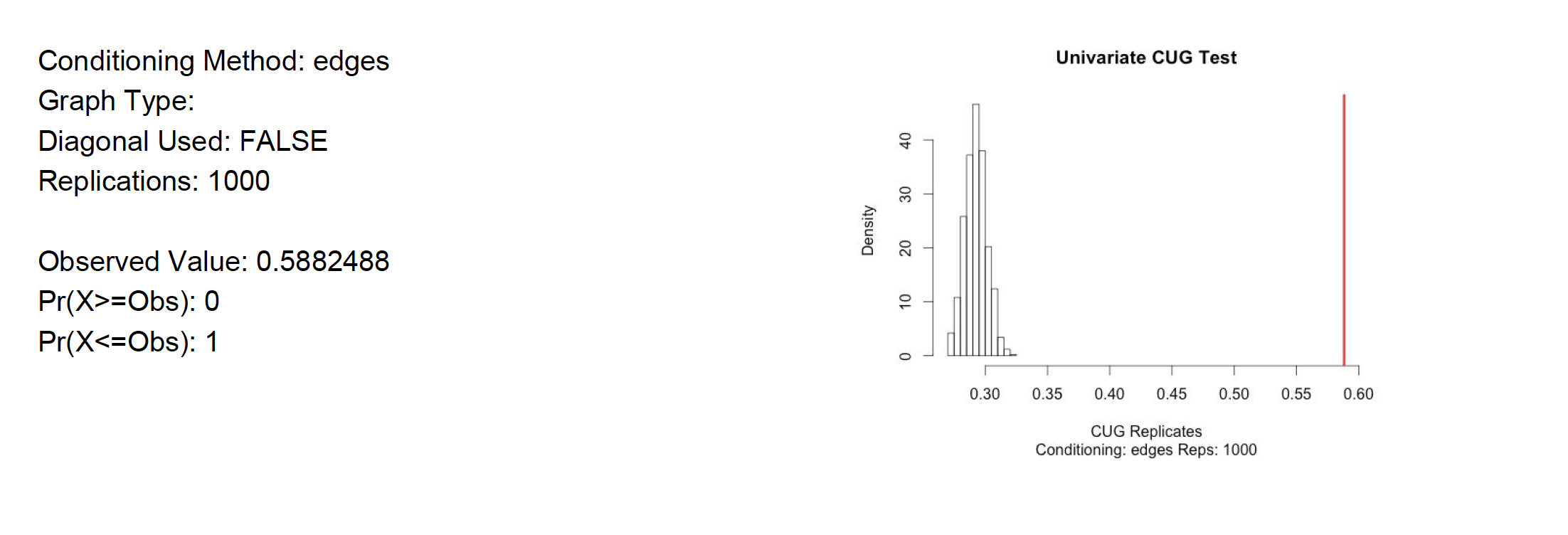
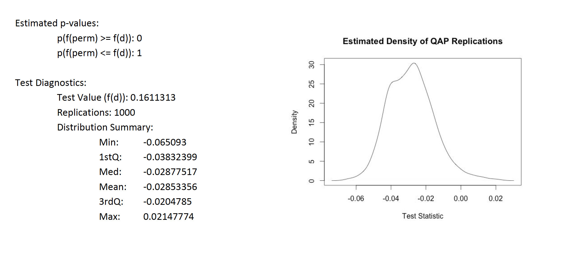
For further analysis Univariate Conditional Uniform Graph Test, CUG, were applied to the filtered user to user projection. The first null hypothesis tested was assortativity with respect to the Rating attribute. Is it similar to that of a random network of the same size and density?. The The null hypothesis is rejected since the assortativity by Rating is close to the average of a random generated network. See test result in appendix A8. However, when testing the null hypothesis by degree assortativity, that states that the user to user network is similar to that of a random network of the same size and density. The hypothesis is rejected. Degree assortativity is much lower than what a random network would show. See appendix A9. All of the randomly generated values are higher than what the user to user network has. In addition, the null hypothesis that the transitivity of the user to user network is similar to that of a random network of the same size and density is also rejected. The user to user network is much higher than any random network. See appendix A10. All of these only proves that the social networks are not random. There is a reason these customer are buying from Amazon instead of going to Barnes & Noble, they are alike and there is not much randomness there. Quadratic Assignment Procedure QAP was also tested on the network. The null hypothesis tested is as follows: the assortativity would be the same regardless the arrangement of the edges. The evidence reject the null hypothesis since all the values are below, that is 100% of the probability mass of test networks has lower assortativity. See appendix A11 for detail.
For further analysis Univariate Conditional Uniform Graph Test, CUG, were applied to the filtered user to user projection. The first null hypothesis tested was assortativity with respect to the Rating attribute. Is it similar to that of a random network of the same size and density?. The The null hypothesis is rejected since the assortativity by Rating is close to the average of a random generated network. See test result in appendix A8. However, when testing the null hypothesis by degree assortativity, that states that the user to user network is similar to that of a random network of the same size and density. The hypothesis is rejected. Degree assortativity is much lower than what a random network would show. See appendix A9. All of the randomly generated values are higher than what the user to user network has. In addition, the null hypothesis that the transitivity of the user to user network is similar to that of a random network of the same size and density is also rejected. The user to user network is much higher than any random network. See appendix A10. All of these only proves that the social networks are not random. There is a reason these customer are buying from Amazon instead of going to Barnes & Noble, they are alike and there is not much randomness there. Quadratic Assignment Procedure QAP was also tested on the network. The null hypothesis tested is as follows: the assortativity would be the same regardless the arrangement of the edges. The evidence reject the null hypothesis since all the values are below, that is 100% of the probability mass of test networks has lower assortativity. See appendix A11 for detail.
Conclusions
Amazon runs a recommender system to provide useful information to customers. One problem is that not every person that buys at the stores provides a rating for the product. Considering that and the fact that Amazon has a huge portfolio of products we know that the space and the networks that may be constructed are very sparse. However, there are techniques that may help identify relevant users. By knowing these users it’s possible to identify products that may be recommended to users in different local networks. These networks have properties that are not common in terms of degree and transitivity. Since the network is very sparse we benefit from the creation of the network to identify thing that in the raw data are not implicit. The edges closeness of users is not evident until the projection is executed. The Amazon book co-purchasing network have local networks that are connected by readers of many categories of book and several clusters of user that have got and rate similar books.
Appendix
A1 - Bipartite Network Summary
IGRAPH UN-B 3147 3602 —
+ attr: name (v/c), Rating (v/n), type (v/c), ERating (e/n)
+ attr: name (v/c), Rating (v/n), type (v/c), ERating (e/n)
A2 - Use to User projection Summary
IGRAPH UNW- 3139 1266475 —
+ attr: name (v/c), Rating (v/n), inDegree (v/n), betweenes (v/n), weight (e/n)
+ attr: name (v/c), Rating (v/n), inDegree (v/n), betweenes (v/n), weight (e/n)
Related posts


