Generalizing Random Forest Model for Online News Popularity Classification

By Mak Hozo, Henna Shah & Julio Sotelo

Abstract

Based on previous work, the Random Forest classifier results in being the most effective algorithm in classifying online news popularity. In this paper, we use this classifier to test its generalizability and robustness across different variations of our data sets. Our results indicated that the algorithm can be generalized successfully but its performance depends significantly on how the data is labeled. It would be useful to use Random Forest to explore other news popularity data sets.

Introduction

Consider the situation where an online news publishing agency is browsing submissions of news articles, but can only accept a few without going over budget or without overwhelming the audience. How does the agency determine which news articles will become popular or even viral, and which news articles will be mostly ignored by the general public? Are there any predictors that indicate how many times an article will be shared amongst audiences? Which articles should the agency purchase and publish?
Implied in this question is the classification problem of binning. Our class variable, the number of shares, is a metric that defines how often an article is shared on social media, but it is a continuous variable and so its binning is not obvious. However, we are interested primarily in articles with high popularity as our positive class, more so than articles with low popularity. So how do we bin a numerical attribute into classes of ‘obscure’, ‘mediocre’, popular’, ‘viral’, etc?
Some previous works in this domain have already identified the technique of random forest to be the best-performing classifier for number of shares (Lei, Hi, Fang 2016). The goal of our analysis is to improve the generalizability of the classifier. How can we take the classifications and apply it to this and other similar data sets to determine when articles will become viral? We accomplish this by looking at the parameters of the classifier such as number of random trees at each split, whether we balance the data, and what our threshold for the high popularity class is.

Data Collection, Preprocessing

To accomplish our analysis, we look at a data set of 39,644 instances of articles published on Mashable.com from 2013 to 2014. The dataset contains 58 total attributes, ranging from the URL of the article, the number of keywords of specific types, what day of the week the article was published, the results of a Latent Dirichlet Allocation algorithm, and the dependent variable: the number of shares of the article. The data set was accessed at the UCI dataset repository referenced in the appendix. There are no missing values in the data set and no significant noise, except for one entry. The 31038th record, about “Ukraine Civilian Convoy Attacked” (from the URL) has values that are impossible to achieve across many variables, such as a rate of 700 in keywords where all other values are less than 1, so we decided to omit this instance. We decided to omit several attributes: five LDA variables and the non-predictive, URL (which included the title and date), and time delta variable. Among the remaining attributes, the non-categorical variables that varied in scale beyond [0,1] were normalized by min-max normalization method.

Furthermore, we analyzed that the distribution of the shares data follows a power law distribution, introducing new challenges to its classification. Based on Figure 1, the majority of the cases center around the median of 1400, with a steep left tail down to 1 share and gradual right tail up to 843,300 shares. As the distribution is heavily skewed to the right, by evaluating the natural logarithm of the shares as shown in Figure 2, we obtain a normal distribution of the class.

Related Work

We have identified Random Forest as being the best performing among several previous works. (Lei, Hi, Fang 2016 and Ren, Yang). The original article that produced the dataset discovered this with an accuracy of 67%, recall of 71%, and AUC of 73% for Random Forest, and lower values for AdaBoost, SVM, KNN, and NB, but a higher precision for Naive Bayes (Fernandes, Vinagre, Cortez 2015). Between RF, SVM, and bagging techniques, Random Forest provides 50.36% accuracy versus 48.0% and 49.97% accuracies of SVM and bagging respectively in another analysis of different techniques (Lee, Hi, Fang 2016). Between a wide variety of algorithms in another article also on the same dataset, Random Forest with 500 trees performed the best with 69% accuracy and 71% recall, outperforming regression and REPTree slightly and SVM, SVR, KNN, and other algorithms by at least 10% (Ren, Yang). Because of these results, we choose to use Random Forest as our classifier for this analysis and focus on our optimization of the technique.

Other studies on the data set tried various ways to classify the dependent variable. For example, the original paper separated the class into two variables with a decision threshold of D_1 = 1400 shares between the high and low popularity classes (Fernandes, Vinagre, Cortez 2015). A second article set four classes having the hig popular ones above 6198 shares (Lee, Hi, Fang 2016). The third article also used a decision threshold of 1400 shares for its binning into two classes (Ren, Yang) while other articles used regression analysis to classify the instances (Dumont, Macdonald, Rincon). On a different data set on Digg scores, one paper received its highest accuracy of 80% by using only 2 classes, and half that for 14 classes (Jamali, Rangwala). A two-class split at the median, 1400 shares, is a good choice for a starting baseline.

Methodology

Since we know that Random Forest is the best performing algorithm to classify popularity of shares, we aim to see how well this classifier can be generalized across different variations of our datasets. In order to achieve this, we decided to look at the following variations of the normalized datasets: the entire dataset with different binning cutoff values, dataset with logarithm of shares as class variable, and subset of the data by looking at cases with shares greater than 10,000, a dataset of about 2223 of the most popular instances. As we have over 39,000 cases, which is more than sufficient for most techniques, we decided to partition the data with a holdout of 66% for the training set and 34% for the testing set.

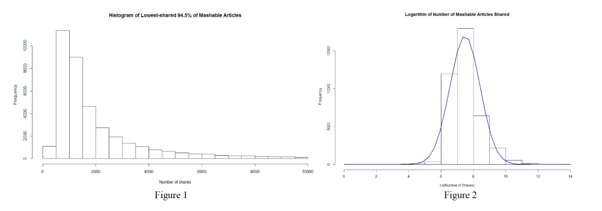
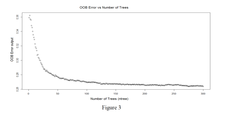
The goal is to see how well the classifier performs in correctly classifying the popular cases, so we limited our classification task to a binary classification problem – whether or not an article is popular. There were various binning techniques used to set the numerical cutoff value to decide how we can label the classes as popular or not popular. For the entire dataset, we used the median value of the shares, 1400, and the third quartile, 2800, as the cutoff values. For the logarithm of shares dataset, we used the median 7.244, and the third quartile 7.937 as our decision boundary for classification. Finally, for the subset of cases with greater than 10,000 shares, we used its median 16,800 and the third quartile 25,300 shares. We also explored a variety of other cutoff values from 1,000 to 100,000 for the full data set and from 11000 to 60000 for the subset of cases greater than 10,000 shares. The resulting plots (see Figure 3) showed no significant change in sensitivity and out of bag error over the entire range. Hence, for the entire dataset, we chose the median, 1400, as our cutoff point for classification as it resulted in balanced classes. This was the same reasoning used in the original paper that provided the dataset (Fernandes, Vinagre, Cortez 2015).

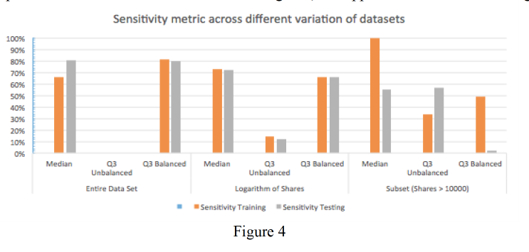
Once the classes were labeled, we looked at the class distribution for each individual combination of dataset and cutoff points. In situations where the class distribution was unbalanced in the training set, we balanced the data using down sampling technique as we had a significant amount of cases. We trained the Random Forest classifier on the balanced and unbalanced training set using different parameters such as the number of random features to be selected at each node (mtry), the number of decision trees the ensemble would contain (ntrees), and setting the “importance” parameter in R to determine the important features. We used an mtry parameter value of 7 based on the guideline of selecting a value that is the square root of the number of attributes, in our case 54. We chose the number of decision trees that minimized the out-of-bag error and number of trees, and followed the law of parsimony – keeping the model simple. Figure 3 indicates a value for ntrees of 150.

After the classifier was trained, it was then applied on the unbalanced testing data to see how the classifier performed. The performance metrics used for our dataset were primarily sensitivity, as we are more interested in knowing how well the classifier performs in correctly classifying the positive class, the popular articles. However, we also included specificity and accuracy in our analysis. The section below extensively explains the results obtained in the training and testing set for different variations of our data sets.

Results

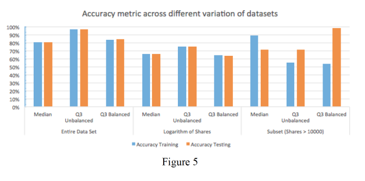
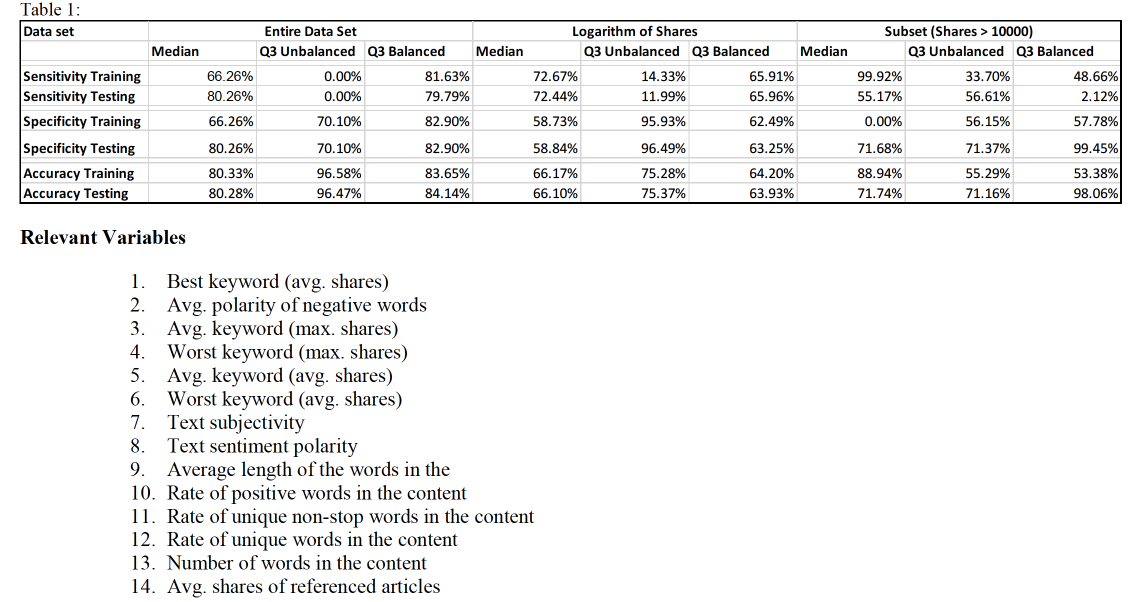
The Table 1 in the appendix shows our results from the analysis. Each data set is represented – the entire data set, the entire data set with the logarithm of the shares column, and the original data set with only the instances where there are more than 10,000 shares. For each data set, the classification label is determined based on the median value and third quartile value for the respective data sets. For all data sets, the third quartile resulted in an unbalanced distribution of classes. Hence, we compared the performance metrics based on the third quartile on unbalanced and balanced training sets, and applied on unbalanced testing sets.

We are primarily focused on evaluating sensitivity and comparing across the models. The classifier achieves a best sensitivity of 72.67% for the training set and 72.44% for the testing set for the data that uses logarithm of shares and median (7.244) as its criteria for partitioning the classes. The actual highest sensitivity is 99.92% in the training set for the subset of data for shares greater than 10,000 where classes are differentiated based on the median. However, it only achieves a 55.17% on the testing data set, which shows severe overfitting. The model is trained specifically to the training data and will not do well on unobserved values. In general, when we look at the entire data set where classes are labeled based on the median, we see a sensitivity of 66.26% on the training set but a higher sensitivity of 80.26% on the testing set. The entire data set performs better because even though it performs the worst on the training set, it performs the best on the testing set. We can conclude that the random forest classifier trained on the entire data set would be the most generalizable classifier.

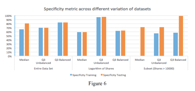
Based on the table, we see that when the labels are classified based on the third quartile value, it results in an unbalanced distribution of classes. Similarly, when the classifiers are trained on the unbalanced data set, it results in very poor sensitivity for training and testing across all data sets. On the other hand, when we balance the class distribution in the training set, we receive sufficiently high sensitivity results in training and testing for the entire data set and the logarithm of shares but for the subsetted data set, we receive a sensitivity of 48.66% in the training and ooly 2.12% in the testing set. This is because the classifier was trained on a balanced training set but tested on an unbalanced testing set, and therefore it could not recognize the minority class, a case of overfitting. The viewer should note that the specificity results for different data sets are present to guide the performance of the unpopular articles if desired. Even though we see high-accuracy results, it is biased towards the majority class and so is not a good measure for our purposes. The three Figures 4, 5, and 6 present each metric for easy comparison across the models.

Relevant Variables

The most important variables identify with the model are related to the keywords used by the articles. Thee top 5 variables to identify popular articles are best keyword (avg. shares), avg. polarity of negative words, avg. keyword (max. shares), worst keyword (max shares), and avg. keyword (avg. shares). For a more complete list see the appendix.

Conclusion and Future Work

The models provided here demonstrate that utilizing a two-class label system with a partition at the median provides what may be the best classifier. The Random Forest classifier can be considered as a generalizable model across different variations of the data set when classes are labeled at the median. This is because even though sensitivity is not very high, the difference between the sensitivity in training and testing set is very low, indicating this model can be used to predict future unknown cases.

When the classifier is trained on datasets with labels set at the third quartile resulting in unbalanced distribution, the classifier has very poor sensitivity – that is, it can not recognize the minority class, the popular articles. However, when the same dataset is balanced, it performs very well in training and unbalanced testing set. In real life, extremely popular instances of viral news articles are very rare (Lee, Hi, Fang 2016). As a result, our dataset does not contain enough cases of popular articles. In fact, it has no online news articles with more than one million shares. Hence, the classifier may not perform as effectively on other datasets.
In order to evaluate the robustness of the Random Forest algorithm, it needs to be applied on different data sets with larger amounts of instances in the high popularity class that can be obtained from different sources. We also need to take into consideration that some of the articles were published less than a month before the data was collected and may not have achieved their full amount of shares. It would be wise to omit those instances, like the original paper recommended (Fernandes, Vinagre, Cortez 2015).

Another algorithm that can be applied to datasets that represent power law distributions would be the Adaboost algorithm that trains decision trees to weigh difficult cases – that is, the high popularity shares. Finally, in order to create better labeling criteria, we can try unsupervised techniques such as K-nearest neighbors, ordered clustering, etc. to help us create labels.

References

• Fernandes, K., Vinagre, P., and Cortez, P.: A Proactive Intelligent Decision Support System for Predicting the Popularity of Online News: Progress in Artificial Intelligence (Springer, 2015), pp. 535-546, http://link.springer.com/chapter/10.1007%2F978-3-319-23485-4_53#page-1, accessed February 12th, 2016.
• Dumont, F., Macdonald, E. B., Rincon, A. F.: Predicting Mashable and Reddit Popularity Using Closed-form and Gradient Descent Linear Regression: COMP598, http://www.ethanbrycemacdonald.com/wp/wp-content/uploads/2015/03/project-1.pdf , accessed February 12th, 2016.
• Lei, X. Hi, X., Fang, H.: Is Your Story Going to Spread Like a Virus? Machine Learning Methods for News Popularity Prediction, http://cs229.stanford.edu/proj2015/326_report.pdf , accessed February 12th, 2016.
• Ee, C. H. C. A. S., & Lim, P. (2001, December). Automated online news classification with personalization. In 4th international conference on asian digital libraries.
  http://citeseerx.ist.psu.edu/viewdoc/download?doi=10.1.1.5.9913&rep=rep1&type=pdf
• Bracewell, D. B., Yan, J., Ren, F., & Kuroiwa, S. (2009). Category classification and topic discovery of japanese and english news articles. Electronic Notes in Theoretical Computer Science, 225, 51-65.
  http://www.sciencedirect.com/science/article/pii/S157106610800529X
• Fernandes, K., Vinagre, P., & Cortez, P. (2015). A Proactive Intelligent Decision Support System for Predicting the Popularity of Online News. InProgress in Artificial Intelligence (pp. 535-546). Springer International Publishing. http://repositorium.sdum.uminho.pt/bitstream/1822/39169/1/main.pdf
• Bandari, R., Asur, S., & Huberman, B. A. (2012). The pulse of news in social media: Forecasting popularity. arXiv preprint arXiv:1202.0332. http://arxiv.org/pdf/1202.0332.pdf
• Tatar, A., de Amorim, M. D., Fdida, S., & Antoniadis, P. (2014). A survey on predicting the popularity of web content. Journal of Internet Services and Applications, 5(1), 1-20. http://link.springer.com/article/10.1186/s13174-014-0008-y
• Hensinger, E., Flaounas, I., & Cristianini, N. (2013). Modelling and predicting news popularity. Pattern Analysis and Applications, 16(4), 623-635. http://link.springer.com/article/10.1007%2Fs10044-012-0314-6
  Ren, H., & Yang, Q. Predicting and Evaluating the Popularity of Online News. http://cs229.stanford.edu/proj2015/328_report.pdf
• Jamali S, Rangwala H (2009) Digging digg: Comment mining, popularity prediction, and social network analysis. In: International Conference on Web Information Systems and Mining (WISM). IEEE, Shanghai, China http://ieeexplore.ieee.org/xpl/articleDetails.jsp?tp=&arnumber=5368318&contentType=Conference+Publications&sortType%3Dasc_p_Sequence%26filter%3DAND(p_IS_Number%3A5367999)%26rowsPerPage%3D50

Appendix